Exploring Regression Models on a Time Series Project

An Educational Overview

In the expansive realm of data science, time series analysis is a vital component, with applications stretching from financial forecasting to weather prediction. This method of analysis focuses on sequences of data points collected over time, which allows us to identify patterns, forecast future occurrences, and make informed decisions based on the analysis of trends [Rafferty, 2021]. What sets time series data apart is the significance of the order in which data points are arranged, as each point is interconnected and informs the next, unlike other types of data where points can be considered independently [Rafferty, 2021]. In this exploration, we delve into the use of non-specialized models, particularly regression models, in our time series project, providing a unique perspective on their application.

The quest to predict the future stretches back centuries and continues to this day, with statisticians and mathematicians enhancing forecasting methods through their discoveries. With each advancement, we come closer to more accurately anticipating events such as market changes, weather patterns, and consumer trends [Taylor & Letham, 2018].

This article will navigate through a variety of statistical techniques that underpin time series analysis. Each of these methods is not only theoretically significant but also offers practical benefits in real-world settings. For example, accurate forecasts can lead to better resource management, strategic business planning, and improved detection of anomalies within systems [Taylor & Letham, 2018]. Another post will detail additional models that are specifically tailored for Time Series dataset problems, such as Facebook Prophet, ARMA, ARIMA, ARDL, and others.

Gaining mastery over time series analysis is crucial for professionals seeking to utilize temporal data effectively. This article will provide insights into techniques such as Ordinary Least Squares (OLS) regression, LASSO, and Ridge regression.

Case Study – Time Series Project using OLS, LASSO, Ridge

We will also delve into a practical case study that highlights the application of these techniques in a real-world scenario. Our project, based on analyzing police department call data, dispositions, and census data within city subzones, serves as a prime example of time series analysis in action. Using a dataset that chronicles the ebb and flow of various metrics over time, we applied statistical methods like OLS regression, LASSO, and Ridge regression to not only understand past trends but also to forecast future occurrences. This case study exemplifies the practical utility of time series analysis in optimizing resource allocation and enhancing public safety strategies.

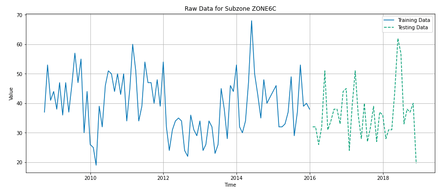
Throughout this guide, references to our project will offer tangible insights into how time series analysis can be effectively utilized in data science. Our project will serve as a continuous thread that connects theoretical concepts with practical implementation.

Understanding Ordinary Least Squares (OLS) Regression in Time Series Projects

Ordinary Least Squares (OLS) regression is recognized for its fundamental role in predictive modeling. It’s a method that seeks the coefficients which minimize the differences between observed values and predictions by squaring these differences and adding them up to form the sum of squared errors (SSE). The goal is to find the line (or hyperplane in multidimensional spaces) that best fits the data, minimizing the SSE to the lowest feasible amount [Kuhn & Johnson, 2013].

The value of OLS lies in the way it quantifies the relationship between variables. OLS coefficients signify the average change in the dependent variable for each one-unit shift in an independent variable, assuming other variables are held steady [Kuhn & Johnson, 2013]. This makes the results from OLS regression straightforward to grasp and interpret, which is why it’s often the first step in data analysis.

However, when using this type of regression model in a time series project, it is important to remember the specific assumptions this model makes, such as the independence of errors, linearity in the relationship between variables, and homoscedasticity (constant variance of errors), which may not always align with the characteristics inherent in time series data. For instance, when time series data comes into play, OLS encounters challenges due to its assumption of independent observations—an assumption that time series data typically violates because each data point may be influenced by previous ones [Rafferty, 2021]. To compensate for this, time series analysis may tweak OLS by integrating techniques such as differencing or implementing error correction models like ARIMA to respect the time-dependent nature of the data.

While it’s clear that OLS regression has its limitations for time series analysis, it remains a valuable preliminary tool. It sets the stage for identifying trends that can be further scrutinized and refined using more specialized time series methodologies. Therefore, OLS is a crucial step in the journey toward understanding and forecasting patterns in data that unfold over time [Rafferty, 2021].

Case Study – Using OLS on the Time Series Dataset

In our project, OLS regression was employed to analyze and predict the trends in police department calls and crime rates within city subzones. We utilized OLS as a foundational model to understand the relationships between various factors—such as census data and police call types—and the frequency of police calls. This approach allowed us to identify potential correlations and average changes in police calls with shifts in different independent variables.

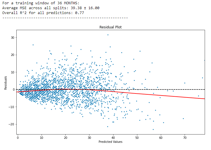
However, given the time series nature of our data, we recognized the limitations of standard OLS regression. Our data, comprising sequential points collected over time, exhibited dependencies between observations. To address this, we adapted our OLS model within a rolling origin framework. This technique involved dividing the dataset into multiple training and testing splits based on time, allowing us to assess the model’s performance over different periods and account for the temporal dependencies inherent in our dataset.

By implementing OLS within this rolling origin approach, we were able to gain preliminary insights into the trends and patterns in our data, setting the stage for more complex and tailored time series analyses. This step proved crucial in our journey to develop models that not only provided a snapshot of past events but also aided in forecasting future occurrences in the realm of public safety and resource allocation.

Thus, in our exploration of time series analysis through this project, OLS regression served as an essential starting point, guiding us towards more intricate methods and models suited for the dynamic nature of time-dependent data.

The Rolling Origin Technique: Enhancing Time Series Predictions

The rolling origin technique stands out as an innovative approach in time series analysis for assessing how well models perform over time. This method, also known as rolling-origin cross-validation or forward-chaining, is carefully designed to respect the sequential and ordered nature of time series data, setting it apart from traditional cross-validation methods which may not account for the temporal dependency inherent in time series data [Rafferty, 2021; Taylor & Letham, 2018].

In practice, the rolling origin technique partitions the dataset into a series of training and testing sets where the testing set is chronologically after the training set. This procedure ensures authenticity in the evaluation process by preventing the model from being influenced by future data when predicting past or current values. The horizon, or the period being predicted, is forecasted after the model is trained on an initial segment of the data. The model’s training window is then expanded to incorporate new data points, and the process repeats [Taylor & Letham, 2018].

This technique mirrors real-world forecasting, where models are continuously updated with new information. By doing so, it offers a robust and reliable means of validating a model’s performance, emphasizing how the model adjusts and responds to changes in data over time. It is a critical step for ensuring models are not only accurate in hindsight but also remain pertinent and effective when faced with new, unseen data [Rafferty, 2021].

Furthermore, the iterative nature of this technique is advantageous for hyperparameter tuning, allowing for a comprehensive assessment of the model’s predictions across different time intervals. Analysts can leverage the insights gained from these evaluations to optimize the model’s settings for superior performance, making the rolling origin technique a cornerstone of effective time series forecasting [Rafferty, 2021].

The rolling origin technique is a key validation tool in the arsenal of time series analysis, ensuring models are robust, adaptable, and prepared for the dynamic nature of real-time forecasting. This methodology is instrumental in achieving more accurate and reliable forecasts and is integral to the model refinement process.

Case Study – How was the rolling origin technique applied?

In our project, the rolling origin technique was a crucial component in analyzing and forecasting the trends observed in police department calls and crime rates in city subzones. Recognizing the importance of capturing the time-dependent nature of our data, we applied this technique to develop and evaluate our predictive models. By applying this technique to our regression models on a time series project, it allows for the validation of model performance over time, accounting for temporal dependencies and providing more realistic forecasts.

Our implementation involved dividing the dataset into a sequence of training and testing sets, each extending forward in time. By training our models on an initial time window and then progressively expanding this window to include new data, we could simulate the real-world scenario of continuously updating models with the latest information. This approach allowed us to assess how well our models predicted future events based on past data, a key aspect of effective forecasting in public safety.

The iterative nature of the rolling origin technique also enabled us to fine-tune our models’ hyperparameters. We could observe how adjustments to these parameters affected the models’ performance over different time periods, leading to optimized settings that enhanced predictive accuracy. This method was particularly beneficial in our project, as it ensured that the models remained robust and adaptable, capable of handling the evolving dynamics of crime rates and police call patterns.

By employing the rolling origin technique, we achieved a more nuanced understanding of our models’ capabilities and limitations. It provided a solid foundation for making reliable predictions, essential for effective resource allocation and strategic planning in public safety management. This method proved invaluable in ensuring that our models were not only accurate in hindsight but also remained relevant and effective when confronted with new, unseen data.

LASSO Regression: Streamlining Regression Models for Time Series

LASSO regression, short for Least Absolute Shrinkage and Selection Operator, presents an evolution in regression analysis. It extends the capabilities of traditional regression by engaging in variable selection and regularization to create models that are both effective and parsimonious. Introduced by Robert Tibshirani in 1996, LASSO is particularly adept at reducing the complexity of a model by penalizing the absolute size of the regression coefficients, and, in some cases, completely eliminating them, setting them to zero [Tibshirani, 1996]. We used the LASSO regression model for prediction in our time series project.

The brilliance of LASSO’s approach lies in its penalty function, which is designed to shrink some coefficients to zero, effectively selecting which variables contribute to the predictive model. This feature is especially beneficial in situations where the dataset includes numerous variables, potentially leading to models that are overly complex and difficult to interpret [Kuhn & Johnson, 2013].

By incorporating regularization, LASSO avoids the pitfalls of overfitting—a common issue where a model learns the noise instead of the signal in the dataset. Regularization in LASSO is achieved through the penalty function, which encourages simpler models that are expected to perform better on new, unseen data. This is essential in time series analysis where overfitting can significantly diminish a model’s forecasting abilities [Rafferty, 2021].

LASSO’s streamlined models not only enhance interpretability but also tend to improve prediction accuracy. By eliminating non-essential predictors, LASSO aims for a sweet spot where the model is complex enough to capture the underlying relationships in the data but not so complex that it loses generalizability [Kuhn & Johnson, 2013].

In summary, LASSO regression emerges as a sophisticated technique for those who prioritize both predictive accuracy and model simplicity. Its unique ability to combine feature selection with regularization makes it a valuable asset for data scientists seeking to build interpretable, efficient, and robust predictive models.

Case Study – Using LASSO regression on the Time Series Dataset

In our project, we employed LASSO regression to analyze the complex dataset comprising police department calls, dispositions, and census data for city subzones. The LASSO model was instrumental in handling the high-dimensional nature of our data, where numerous variables could potentially impact the number and types of police calls.

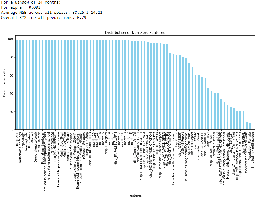
LASSO’s ability to perform variable selection was particularly valuable in our context. It helped us identify the most relevant predictors from a broad range of variables, including demographic data, historical crime rates, and various socio-economic indicators. By penalizing the absolute size of the regression coefficients, LASSO simplified our model, reducing the risk of overfitting and enhancing its interpretability. This feature was crucial for our project, as it allowed us to focus on the most significant factors influencing police calls and crime rates, ensuring that our model remained robust and relevant.

Additionally, the regularization aspect of LASSO proved vital in maintaining the model’s predictive accuracy. It helped us balance the complexity of the model with the need for generalizability, ensuring that our predictions were not just a reflection of the noise in our training data but also applicable to new, unseen data. This aspect was particularly crucial for our objective of forecasting future trends in police calls and crime rates, as it improved the model’s reliability and effectiveness in real-world scenarios.

Through the application of LASSO regression, our project successfully navigated the challenges of a complex, high-dimensional dataset, resulting in a model that was not only accurate in its predictions but also straightforward in its interpretation. LASSO’s blend of feature selection and regularization made it an indispensable tool in our analysis, highlighting its efficacy in time series forecasting within the realm of public safety. Once again, while this regression model on our time series dataset was able to accurately account for about 80% of the variation in our target feature, there are still better regression models for this application. Next we will explore the use of ridge regression.

Ridge Regression: Tackling Overfitting in Time Series ModelingA Solution to Overfitting in Predictive Models

Ridge regression emerges as a formidable approach to predictive modeling, specifically crafted to mitigate overfitting. Overfitting is a scenario where a model learns the random fluctuations of the training data rather than the actual trend, which can degrade the model’s performance on new, unseen data. Ridge regression addresses this by penalizing the magnitude of the coefficients, compressing them towards zero but crucially, without ever setting them to zero, as LASSO regression might [Hoerl, 1970; Kuhn & Johnson, 2013].

The key distinction between Ridge and LASSO regression is their penalty mechanisms. Ridge regression applies an L2 penalty, squaring the coefficient values, whereas LASSO employs an L1 penalty that takes their absolute values. This subtle difference means that Ridge regression preserves all the predictors in the model, although with diminished weights, which is advantageous when dealing with multicollinearity—a condition where independent variables are highly interrelated [Kuhn & Johnson, 2013].

Multicollinearity can cause inflated and unstable estimates of regression coefficients, undermining the model’s predictive accuracy. Ridge regression effectively dilutes the impact of multicollinearity by allowing correlated predictors to share strength, leading to more reliable coefficient estimates. This is particularly beneficial when the number of predictors is high, potentially surpassing the number of observations [Kuhn & Johnson, 2013].

Additionally, the calibration of a hyperparameter, typically represented by lambda (λ), is a critical step in Ridge regression. This hyperparameter controls the severity of the penalty and must be optimized to strike a balance between bias and variance in the model. Techniques like cross-validation are instrumental in determining the ideal λ value, ensuring the model is attuned for the best predictive performance on new data [Kuhn & Johnson, 2013].

Ridge regression is thus a valuable technique for those aiming to create dependable predictive models. Its comprehensive approach to preventing overfitting, without eliminating any variables, makes it particularly suitable for complex datasets where predictors may be closely intertwined.

Case Study – Using Ridge Regression on the Time Series Dataset

In our project, Ridge regression played a role in modeling the intricate relationships within our dataset, which included various factors like census data, historical crime rates, and police call types. Given the high dimensionality and potential multicollinearity within our time series data, Ridge regression was particularly apt for our analysis.

We opted for Ridge regression due to its ability to handle multicollinearity effectively. The interrelated nature of our predictors, such as socio-economic indicators and demographic variables, could have led to unstable coefficient estimates in a regular OLS model. Ridge regression, with its L2 penalty, allowed us to include all these predictors while controlling for multicollinearity, thus ensuring that our model remained stable and reliable.

The tuning of the lambda (λ) parameter in Ridge regression was a critical aspect of our model development process. Through cross-validation, we optimized λ to find the ideal balance that minimized overfitting while retaining the model’s predictive power. This step was crucial in enhancing the model’s performance, particularly in forecasting future police calls and crime rates based on past trends and patterns.

Ridge regression’s comprehensive approach enabled us to develop a model that was robust against overfitting and capable of providing reliable forecasts. This was vital for our objective of creating a predictive tool that could aid in effective resource allocation and strategic planning for public safety.

Thus, in our endeavor to build a predictive model for time series data, Ridge regression emerged as an essential technique. Its ability to manage complex datasets with numerous interrelated variables made it a suitable choice for our project, underscoring its value in creating dependable and effective predictive models in the field of data science.

Optimizing Model Performance: The Role of Cross-Validation and Grid Search

Cross-validation and grid search are pivotal in refining the performance of statistical models, notably within the realms of LASSO and Ridge regression. Cross-validation serves to validate the model’s effectiveness, offering a more reliable measure of its predictive power by using different subsets of the data for training and testing [Kuhn & Johnson, 2013]. This is particularly crucial in time series analysis, where the sequence of data points cannot be shuffled due to their chronological order. Rolling-origin cross-validation, a variant suited for time series, ensures that the model is tested on future data points, maintaining the temporal integrity of the dataset [Rafferty, 2021].

Grid search complements cross-validation by exhaustively searching through a predefined range of hyperparameter values to identify the combination that delivers the best predictive accuracy. It is a systematic approach to hyperparameter tuning, vital for refining the regularization strength in LASSO and Ridge regression models. The interplay between these models’ penalty terms and their predictive performance is delicately balanced through grid search, guided by cross-validation results [Rafferty, 2021].

While grid search is thorough, it can be resource-intensive. Alternative strategies like random search provide a more computationally efficient solution without significantly compromising the quality of results [Santu et al., 2020]. Advanced techniques like Bayesian optimization further streamline the tuning process by applying probabilistic models to predict the performance of hyperparameters, thus focusing on the most promising regions of the hyperparameter space [Santu et al., 2020].

The thoughtful application of cross-validation and grid search in model tuning is not just a matter of academic interest but a practical necessity. It anchors the predictive capabilities of LASSO and Ridge regression models in reality, ensuring that they are not just statistical constructs but effective tools for forecasting and analysis.

Case Study – How we applied CV and GridSearch

In our project, cross-validation and grid search were instrumental in refining the performance of our LASSO and Ridge regression models. We employed rolling-origin cross-validation, a technique particularly well-suited for time series data like ours. This method allowed us to maintain the chronological order of the data, ensuring that our models were tested on future data points, thus providing a realistic measure of their predictive capabilities.

Grid search played a critical role in our hyperparameter tuning process. By systematically exploring a range of values for the regularization strength in our LASSO and Ridge models, we identified the optimal settings that balanced the complexity of the model with its predictive accuracy. This exhaustive search, though computationally demanding, was crucial in determining the most effective lambda (λ) values for our models.

In addition to grid search, we also explored more computationally efficient methods like random search, which offered a quicker yet effective way to navigate the hyperparameter space. This approach was particularly beneficial given the large size and complexity of our dataset, enabling us to efficiently fine-tune our models without extensive computational resources.

The application of these techniques ensured that our models were not only statistically sound but also practically effective. By rigorously testing and tuning our LASSO and Ridge regression models, we developed robust forecasting tools capable of providing accurate predictions for police calls and crime rates. This optimization process was vital in ensuring that our models could reliably inform decision-making processes and resource allocation strategies in public safety management.

Through cross-validation and grid search, we were able to bridge the gap between theoretical modeling and practical application, demonstrating the real-world efficacy of our time series analysis in the context of public safety. The integration of these techniques was vital in optimizing the performance of our regression models on this time series project. Should we expand our analysis to include advanced time series models such as ARMA, ARIMA, ARDL, or Facebook Prophet, the use of cross-validation and grid search would become even more paramount. These models possess a multitude of hyperparameters, and their careful tuning is crucial to harness their full potential and ensure the most accurate and reliable forecasts for our dataset.

Residual Analysis: Assessing Model Fit and Accuracy

When delving into the world of predictive modeling, residual analysis emerges as a pivotal aspect of evaluating a model’s performance. Residuals, essentially the discrepancies between the observed data points and the predictions generated by the model, serve as a barometer for gauging how accurately the model reflects the data it’s intended to represent [Kuhn & Johnson, 2013].

Engaging in residual analysis is akin to having a diagnostic check-up for your model. By scrutinizing these residuals, significant insights can be unearthed about the model’s effectiveness. Plots of residuals versus fitted values are particularly telling; they should ideally display a random cloud of points, indicating that the model’s predictions are unbiased. A discernible pattern in this plot could signal that the model is not capturing some aspect of the data’s structure [Kuhn & Johnson, 2013].

Moreover, residual analysis can detect anomalies such as outliers or influential observations that might skew the model’s parameters. It is crucial to identify such data points as they could indicate that further data cleansing or transformation may be necessary to improve the model’s performance [Kuhn & Johnson, 2013].

In essence, the examination of residuals is not a mere academic exercise but a practical step towards refining model accuracy. It is an essential practice for any data scientist aiming to build predictive models that not only fit the historical data but are also robust and reliable for making future forecasts.

Case Study – Residual Analysis was crucial in Evaluating the Models

In our project, residual analysis played a crucial role in assessing the fit and accuracy of our predictive models, including the OLS, LASSO, and Ridge regression models on this time series dataset. We meticulously examined the residuals – the differences between our models’ predictions and the actual observed values – to gauge how well our models captured the underlying patterns in the data.

We created plots of residuals against fitted values for each model. These plots were instrumental in revealing whether our models were biased or if there were any patterns left unexplained. Ideally, we expected to see a random dispersion of points, suggesting that our models were accurately capturing the essential dynamics of the data. Any discernible patterns or trends in these plots would indicate a model misspecification, prompting us to revisit our model selection or consider additional data transformations.

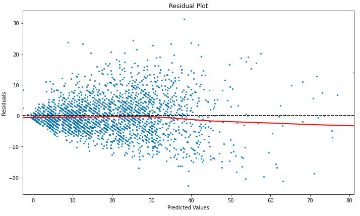
Additionally, we used residual analysis to identify outliers and influential data points that could potentially distort our models’ predictions. This step was vital for ensuring the robustness of our models. It helped us determine whether these points were anomalies or indicative of underlying trends not captured by our models. In some cases, this led to further data cleansing or the introduction of additional variables to enhance the models’ predictive power.

Through this comprehensive residual analysis, we were able to refine our models significantly. It enabled us to develop predictive tools that were not just statistically sound but also practically effective.

Bootstrapping for Reliable Prediction Intervals

The bootstrap method is a powerful statistical tool that enables the estimation of prediction intervals, which are essential for understanding the uncertainty inherent in any model prediction. This resampling technique involves repeatedly drawing samples, with replacement, from the original dataset to create numerous “bootstrap” datasets. Models are then fitted to these datasets, and from the variation in the predictions across these models, prediction intervals can be constructed [Efron and Tibshirani, 1986; Kuhn & Johnson, 2013].

Prediction intervals offer a range of values within which we can expect future observations to fall, at a given probability level. They provide a quantifiable measure of the uncertainty in predictions, which is crucial for risk assessment in decision-making processes. Without such intervals, a single point estimate gives a false sense of certainty, ignoring the potential variability in future outcomes [Kuhn & Johnson, 2013].

Moreover, bootstrapped prediction intervals can be particularly informative when comparing models. For instance, if two models’ prediction intervals significantly overlap, it may suggest that there is no statistical difference in their performance, which could guide the selection of a simpler or more interpretable model [Kuhn & Johnson, 2013].

One of the advantages of bootstrapping is that it does not make rigid assumptions about the distribution of the data, making it a flexible approach suitable for a wide range of applications. However, it is important to recognize that bootstrapping can be computationally intensive, and its reliability depends on the size of the original dataset. Large enough datasets are needed to ensure a representative range of samples is drawn during the resampling process [Kuhn & Johnson, 2013].

Bootstrapping is an indispensable method for estimating reliable prediction intervals in regression analysis. It underscores the importance of acknowledging and quantifying uncertainty, allowing for more informed and risk-aware decisions based on model predictions.

Case Study – Bootstrapping to Find Prediction Intervals

In our project, we utilized the bootstrap method to estimate prediction intervals for our time series models, including the LASSO and Ridge regression models. This approach was critical in quantifying the uncertainty in our forecasts of police calls and crime rates. By creating numerous bootstrap samples from our original dataset and fitting models to each of these samples, we were able to observe the variability in the predictions.

The generation of prediction intervals through bootstrapping gave us valuable insights into the range of possible outcomes. This was especially important for our project, as it allowed us to assess the risk and potential variability in future police call and crime rate predictions. Understanding this uncertainty was crucial for planning and resource allocation in public safety management.

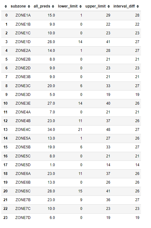
Furthermore, the bootstrapped prediction intervals aided in the comparative analysis of our models. By examining the overlap of prediction intervals between different models, we gained a deeper understanding of their relative performance. This analysis was pivotal in guiding our decision-making process, helping us choose models that not only provided accurate forecasts but also accounted for uncertainty in a realistic and practical manner.

While bootstrapping is a computationally intensive technique, its flexibility and non-reliance on strict assumptions about data distribution made it well-suited for our complex and high-dimensional dataset. The size of our dataset allowed for a comprehensive and representative range of samples in the resampling process, enhancing the reliability of the prediction intervals.

By employing bootstrapping in our regression models on time series project, we were able to provide a more nuanced picture of our models’ predictive capabilities, enhancing our understanding of prediction uncertainty. This method not only underscored the importance of considering uncertainty in our forecasts but also ensured that our predictive models were robust and aligned with the practical realities of forecasting in the field of public safety. The use of bootstrapping highlights the intricate balance between precision and practicality that is essential when applying regression models to complex time series data, contributing significantly to the reliability and effectiveness of our analysis.

Exploring the Impact of Feature Selection on Predictive Models

Feature selection is a pivotal step in the construction of predictive models, primarily aiming to enhance model accuracy and provide insight into the key drivers behind the data. LASSO (Least Absolute Shrinkage and Selection Operator) and Ridge regression are two widely implemented techniques that serve this goal. They tackle overfitting—a common pitfall where a model performs well on training data but fails to generalize to unseen data—and highlight the most influential variables.

The key differentiation between LASSO and Ridge regression lies in how they manage multicollinearity, which occurs when multiple features are closely intertwined. Ridge regression reduces the volatility of the coefficient estimates by imposing a penalty on the size of coefficients, effectively pulling them towards each other but not to zero, thus retaining all features in the model [Kuhn & Johnson, 2013]. Conversely, LASSO goes a step further by potentially zeroing out the coefficients of less critical predictors, thereby naturally performing feature selection and yielding a more streamlined model that highlights only the essential predictors [Kuhn & Johnson, 2013].

These penalization methods—Ridge applying a penalty on the square of the coefficients and LASSO on their absolute values—have distinctive implications on the resulting models. While Ridge regression tends to maintain a more complex model with numerous small, non-zero coefficients, LASSO favors simplicity and interpretability by allowing the exclusion of certain features altogether [Kuhn & Johnson, 2013].

Understanding the importance of feature selection extends beyond academic interest; it has tangible benefits in various industries. In healthcare, for instance, focusing on critical patient data can significantly improve the accuracy and interpretability of diagnostic models, thereby supporting physicians in clinical decision-making. In the financial sector, recognizing which factors heavily influence asset prices can refine investment strategies and yield better financial outcomes.

To sum up, employing feature selection through methods like LASSO and Ridge regression models on our time series project not only improves the predictive strength of models but also contributes to their simplicity and intelligibility. This approach leads to the creation of streamlined, effective models that facilitate more informed decision-making across diverse sectors, demonstrating the practical advantages of applying these regression techniques in time series analysis.

Visualizing Uncertainty in Model Predictions

Interpreting predictions from our regression models on time series project becomes substantially more meaningful when the associated uncertainty is clearly communicated. Error bars serve as an effective visual tool to represent prediction intervals in regression models, offering a glimpse into the range within which the true outcome is likely to occur, as per a designated probability level [Taylor & Letham, 2018].

Incorporating error bars into model visualizations equips stakeholders with a clearer understanding of potential outcomes and the risks entailed. This is particularly useful in domains such as business forecasting, where comprehending the scope of uncertainty is fundamental for decision-makers [Rafferty, 2021].

Furthermore, error bars can be indicative of a model’s robustness. A model suffering from overfitting, which is characterized by narrow error bars on training data and disproportionately wide intervals for predictions, can be promptly identified and rectified [Taylor & Letham, 2018]. Such visual clues are invaluable for analysts who strive to enhance the model’s predictive accuracy and generalizability.

The default uncertainty interval in tools like Prophet is typically set at 80%, although this can be adjusted to reflect varying levels of confidence, such as a 95% interval for more conservative scenarios. Modifying the uncertainty interval allows for tailored visualizations that match the risk appetite of the decision-makers [Rafferty, 2021].

Visualizing uncertainty is not only beneficial for effective communication but also acts as a diagnostic measure for improving model performance. By delineating the expected variability in predictions, stakeholders can assess the trustworthiness of the model’s forecasts and make decisions that align with their accepted level of risk.

In our project, visualizing uncertainty played a critical role in interpreting the predictions from our time series models. By incorporating error bars into our visualizations, we were able to effectively communicate the uncertainty associated with the predictions of police calls and crime rates. These error bars, representing prediction intervals, provided a clear indication of the range within which we could expect actual future values to fall.

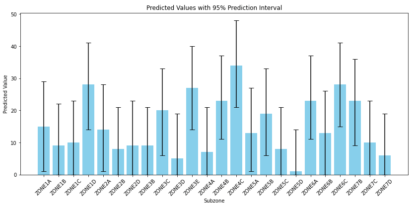
We utilized error bars in our LASSO and Ridge regression model outputs, allowing stakeholders to understand not just the predicted values but also the confidence level surrounding these predictions. This approach was especially valuable in the context of public safety planning, where decision-makers needed to gauge the reliability of our forecasts and prepare for a range of potential outcomes.

Moreover, the process of feature selection, guided by LASSO and Ridge regression, directly influenced the uncertainty in our model predictions. By selecting the most relevant features and appropriately penalizing others, we were able to refine our models, which was reflected in the precision of our prediction intervals. Narrower error bars on our training data suggested a good fit, while the intervals for predictions provided insights into the models’ generalizability to unseen data.

We also adjusted the uncertainty intervals based on the risk preferences of our stakeholders. In scenarios requiring more conservative approaches, we increased the confidence interval, such as setting it at 95%, to encompass a broader range of potential outcomes. This flexibility allowed us to tailor our visualizations and predictions to the specific needs and risk tolerance of our audience.

The visualization of uncertainty through error bars was not only a means of effective communication but also a crucial aspect of our model evaluation process. It helped us identify areas for improvement in our models and provided a tangible way for stakeholders to understand and trust our predictions. The integration of feature selection techniques further enhanced this process, contributing to the development of robust, reliable, and interpretable predictive models for public safety management.

Conclusion

Through analysis and comparison using various visualizations and tables, we were able to indepthly evaluate these regression models used in our time series project. We observed that the Ridge Regression model slightly outperformed its counterparts in LASSO and OLS regression. Notably, the Ridge model demonstrated a robust R-Squared value of 79%, indicating its strong ability to capture the variance in the response variable. This was complemented by a lower mean squared error compared to the other models, suggesting greater accuracy in predictions.

The distinction between the L1 regularization in LASSO and the L2 regularization in Ridge Regression, although subtle, proved significant in our analysis. Ridge Regression, with its smaller deviations, not only offered more accurate predictions but also maintained a simplicity that prevented model overcomplexity. This balance was particularly evident in the visualization of prediction intervals, which, while slightly wider, did not compromise the model’s interpretability.

Our final model, used for predicting January 2019’s crime rates, encapsulates the effectiveness of Ridge Regression in handling such complex time series data. It’s crucial to note that while the model explains a substantial portion of the variance, the actual predicted values for January 2019 remain unverified. Nonetheless, the model’s performance during the training and testing phases instills confidence in its predictive capabilities.

In summary, this exploration of OLS, LASSO, and Ridge Regression, grounded in a real-world application, underscores the importance of choosing the right model and fine-tuning it to the data at hand. Our case study reinforces the idea that in data science, especially in time series analysis, the path to accurate forecasting is paved with meticulous model selection, careful evaluation, and an appreciation of the subtleties that differentiate various modeling approaches. In the end, our chosen models were for an educational goal, rather than an actual business objective. There are other models that would potentially perform better on this dataset, and others like it.

References

• Efron, B., & Tibshirani, R. J. (1986). Bootstrap methods for standard errors, confidence intervals, and other measures of statistical accuracy. Statistical Science, 1(1), 54-75.
• Hoerl, A. E. (1970). Ridge regression: Biased estimation for nonorthogonal problems. Technometrics, 12(1), 55-67.
• Kuhn, M., & Johnson, K. (2013). Applied Predictive Modeling (Vol. 26, p. 13). New York: Springer.
• Rafferty, G. (2021). Forecasting Time Series Data with Facebook Prophet: Build, improve, and optimize time series forecasting models using the advanced forecasting tool. Packt Publishing Ltd.
• Santu, S. K. K., Hassan, M. M., Smith, M. J., Xu, L., Zhai, C., & Veeramachaneni, K. (2020). AutoML to Date and Beyond: Challenges and Opportunities. arXiv preprint arXiv:2010.10777.
• Taylor, S. J., & Letham, B. (2018). Forecasting at scale. The American Statistician, 72(1), 37-45.
• Tibshirani, R. (1996). Regression shrinkage and selection via the lasso. Journal of the Royal Statistical Society: Series B (Methodological), 58(1), 267-288.